Brier Score Explained: Formula, Interpretation, and Code
The Brier score measures the mean squared difference between a predicted probability and what actually happened, scored as 0 or 1. For binary events, the formula is BS = (1/N) Σ(ft − ot)², where ft is the forecast probability and ot is the observed outcome. Lower is always better, with 0 marking a perfect forecast and 1 marking the worst possible one.
A single number, though, hides more than it reveals. The Brier score bundles two separate skills together: how well-calibrated your probabilities are and how well they discriminate between outcomes that happen and those that don’t. That’s why the score should never be judged in isolation. The Murphy decomposition splits it into reliability, resolution, and uncertainty, and the Brier Skill Score puts it in context against a baseline. Both get a full walkthrough below, along with a worked example and code you can run yourself.
- Formula: BS = (1/N) Σ(ft − ot)²
- Range: 0 (perfect) to 1 (worst) for binary forecasts
- Rule type: a strictly proper scoring rule, meaning honest probability estimates minimize expected score
- Practical takeaway: decompose before you judge — a “good” score can still hide bad calibration
Key Takeaways
The Brier score measures forecast accuracy as mean squared error between predicted probability and outcome, and it only becomes meaningful once decomposed into reliability, resolution, and uncertainty.
| Point | Details |
|---|---|
| Core formula | Binary Brier score equals the average of (predicted probability minus outcome) squared across all forecasts. |
| Lower is better | Scores range from 0 (perfect) to 1 for binary events, with no universal “good” threshold. |
| Decompose before judging | Split the score into reliability, resolution, and uncertainty to see whether error comes from calibration or task difficulty. |
| Use BSS for comparisons | The Brier Skill Score measures improvement over a base-rate reference and enables comparison across datasets. |
| Betsyscore applies this live | Betsyscore’s win-probability forecasts run on the same calibration logic, tracked per match and rolled into daily BSS monitoring. |
Table of Contents
- What Is the Brier Score in Statistics?
- Worked Example: How to Calculate the Brier Score
- Why Does Decomposition Matter for the Brier Score?
- How Do You Calculate a Brier Skill Score?
- Common Misconceptions and Pitfalls With the Brier Score
- What Counts as a Good Brier Score?
- How to Compute the Brier Score in Python and R
- Where Is the Brier Score Used in Practice?
- What Are the Limitations of the Brier Score?
- How BetsyScore Monitors Prediction Quality in Production
- A Practitioner’s Priority List for Using the Brier Score
- See Real-Time Probabilistic Forecasts in Action
- Sources
- FAQ
What Is the Brier Score in Statistics?
The Brier score in statistics is a proper scoring rule built for evaluating probabilistic forecasts against binary or categorical outcomes. It was introduced by meteorologist Glenn W. Brier in 1950 to grade weather forecasters on how well their stated rain probabilities matched what actually fell from the sky, and the same math now grades everything from spam filters to injury-risk models.
Binary formula:
BS = (1/N) Σ(ft − ot)²
- N is the number of forecast-outcome pairs.
- ft is the predicted probability for event t, between 0 and 1.
- ot is the actual outcome for event t, either 0 (did not happen) or 1 (happened).
Notice this is exactly the mean squared error you’d compute for any regression problem, just applied to probabilities predicting a binary target. That equivalence matters because it means every tool built for MSE, from gradient descent to bootstrap confidence intervals, applies directly to Brier scores without modification.
Multi-class extension, used when an event has more than two possible outcomes (say, win/draw/loss in a football match):
BS = (1/N) Σt Σi (fti − oti)²
Here the inner sum runs across all R possible categories i for each forecast t, comparing the predicted probability for each category against a one-hot indicator of what actually happened. This changes the numeric range: instead of capping at 1, the original multi-category formulation caps at 2, per the UVA Library’s breakdown, because the squared errors accumulate across every category rather than just one.
- Binary Brier score range: 0 to 1
- Multi-category Brier score range: 0 to 2 (in the original formulation)
- Some libraries rescale multi-class output, so always check documentation before comparing numbers across tools
Why is it “proper”? A proper scoring rule is one where a forecaster minimizes their expected score by reporting their true belief, not a strategically hedged number. If you secretly believe there’s a 70% chance of an event but report 90% to look confident, your expected Brier score gets worse, not better. That property is what makes the metric trustworthy for evaluating forecasters and models alike, rather than just accuracy checkers.
One scaling quirk trips up a lot of newcomers: scikit-learn’s brier_score_loss uses the standard binary [0,1] convention, but some academic papers divide the multi-class sum by two to force a [0,1] range. Check which convention a paper or library uses before comparing scores across sources.
Worked Example: How to Calculate the Brier Score
Here’s a small forecasting exercise: predicting whether five football matches end in a home win. The table shows each predicted probability, the actual outcome, and the squared error contribution.

Sum the squared errors and divide by the number of predictions to calculate the Brier score, which in this example indicates reasonably good forecast accuracy.
That 0.1205 sits closer to the “perfect” end of the 0 to 1 scale, meaning the forecasts tracked reality reasonably well across these five matches. A few edge cases worth knowing:
- A forecaster who nails every outcome with 100% confidence scores a perfect 0.
- Always predicting the base rate (say, 45% home wins if that’s the historical average) produces a stable, moderate score that resists big penalties but also never approaches 0.
- Predicting 0.99 on an event that doesn’t happen produces a squared error near 0.98, close to the maximum penalty. Extreme confidence is punished hard when it’s wrong.
Why Does Decomposition Matter for the Brier Score?
A single Brier score can’t tell you whether your model is well-calibrated, sharp, or just lucky given the data’s natural difficulty. Murphy’s decomposition breaks it into three additive components that answer that question directly:
BS = Reliability − Resolution + Uncertainty
- Reliability (calibration): how closely predicted probabilities match observed frequencies. If you predict 70% across a batch of events and 70% of them actually occur, reliability error is near zero. Lower reliability values are better here, since this term measures miscalibration.
- Resolution: how much your forecasts vary from the overall base rate and still turn out to be right. High resolution means your model separates likely events from unlikely ones instead of hedging toward the average. Higher resolution is better, and it’s subtracted in the formula.
- Uncertainty: the irreducible variance in the outcome itself, determined purely by the base rate. If 50% of matches end in a home win, uncertainty is at its mathematical maximum; if only 5% do, uncertainty shrinks regardless of forecasting skill.
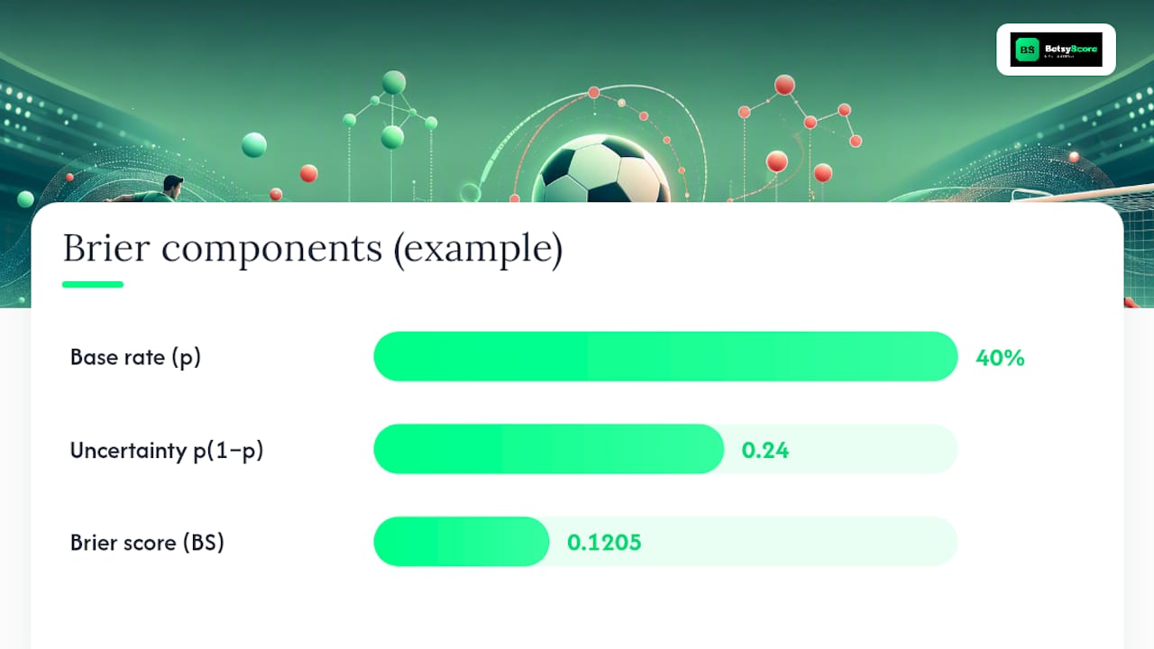
Applying this to the five-match example: if the base rate of home wins in the historical dataset is 40%, uncertainty is fixed by that rate alone, roughly 0.24 (calculated as p(1−p)). The remaining gap between the overall Brier score of 0.1205 and that uncertainty term reflects the balance of reliability and resolution, meaning most of this model’s error traces back to imperfect calibration rather than the task’s inherent difficulty.
This is the practical warning worth repeating: two models can post an identical headline Brier score of, say, 0.15, while one has excellent calibration and poor resolution (it hedges toward the base rate and rarely commits) and the other has strong resolution but shaky calibration (it makes bold, differentiated calls that run systematically too confident). Only the decomposition exposes that difference, and pairing it with a calibration curve, a plot of predicted probability against observed frequency, makes the diagnosis visual.
How Do You Calculate a Brier Skill Score?
The Brier Skill Score converts a raw Brier score into a relative measure of improvement over some baseline, which solves the biggest headache with reading Brier scores cold: they can’t be compared across tasks with different base rates. The formula is:
BSS = 1 − (BS_model / BS_reference)
The reference is almost always a climatology or base-rate predictor, a model that always forecasts the historical average probability of the event, ignoring all case-specific information. For football, that might mean always predicting the season-wide home win percentage regardless of the two teams involved.
- BSS > 0: your model beats the baseline, meaning it performs better than simply guessing the average event probability.
- BSS = 0: your model performs no better than always predicting the base rate, a red flag that your added complexity isn’t earning its keep.
- BSS < 0: your model is actively worse than the naive baseline, which happens more often than practitioners expect when a model overfits or gets deployed on a shifted population.
Choosing the right reference matters more than most guides admit. Climatology works for weather and long-running sports leagues with stable historical rates. For a newly promoted team with no track record, or a rare event like a red card in the first five minutes, a naive base-rate reference can be misleading, and picking a more recent or narrower comparison window often gives a fairer skill read.
Common Misconceptions and Pitfalls With the Brier Score
The single biggest misconception is that there’s a universal cutoff for a “good” Brier score. There isn’t. A score of 0.20 might be excellent for a highly unpredictable event and mediocre for one with a lopsided base rate.
- Mistake: assuming a low score means good calibration. A model that always predicts the base rate can post a deceptively low score purely because uncertainty is small, not because it’s actually skillful. Corrective action: run the Murphy decomposition and check resolution separately.
- Mistake: comparing scores across datasets with different base rates. A Brier score of 0.10 on a 50/50 event is far more impressive than 0.10 on a 90/10 event. Corrective action: use the Brier Skill Score against a matched baseline instead of the raw number.
- Mistake: treating the Brier score as a complete evaluation. Peer-reviewed discussions of forecast evaluation caution against relying on any single scalar metric, recommending calibration curves and decomposition alongside the headline figure.
Pro Tip: Never report a bare Brier score in a model comparison table without also stating the base rate of the event and, ideally, the BSS against a matched reference. The number alone invites the wrong conclusion.
What Counts as a Good Brier Score?
There’s no fixed threshold, since the “goodness” of a Brier score depends entirely on the base rate and difficulty of the event you’re forecasting.
- Run the full decomposition first. Separate reliability from resolution before deciding if a score reflects genuine skill or lucky calibration against a stable base rate.
- Plot a calibration curve. Bin your predictions (0 to 10%, 10 to 20%, and so on) and check whether observed frequencies track predicted probabilities in each bin.
- Compute the Brier Skill Score against a sensible reference. A climatology or base-rate baseline turns an unreadable absolute number into a comparable improvement percentage.
- Use bootstrapped confidence intervals. Resampling your forecast-outcome pairs shows whether an apparent improvement between two models is statistically meaningful or noise.
- Compare models on identical data. Never compare a Brier score from one season, league, or dataset directly against another without adjusting for differing base rates.
How to Compute the Brier Score in Python and R
Computing a Brier score from scratch takes one line of vectorized code in either language, and both ecosystems have tested libraries so you don’t have to trust your own arithmetic.
Python, using scikit-learn’s brier_score_loss:
import numpy as np
from sklearn.metrics import brier_score_loss

y_true = np.array([1, 0, 1, 0, 0])
y_prob = np.array([0.80, 0.30, 0.60, 0.10, 0.55])

bs = brier_score_loss(y_true, y_prob)
print(f"Brier score: {bs:.4f}")
This reproduces the 0.1205 result from the worked example above, since brier_score_loss applies the same mean-squared-error formula under the hood.
R, using base functions, with scaled-Brier logic drawn from Clinicalpredictionmodels:
y_true <- c(1, 0, 1, 0, 0)
y_prob <- c(0.80, 0.30, 0.60, 0.10, 0.55)

brier_score <- mean((y_prob - y_true)^2)
cat("Brier score:", round(brier_score, 4), "
")
Pro Tip: For multi-class problems, confirm whether your library sums squared errors across all categories (range up to 2) or averages them (range up to 1) before comparing scores between tools. Mixing conventions is the most common source of “my Brier score looks wrong” bug reports.
For decomposition and calibration plots, keep bin counts large enough that each probability bucket has a meaningful sample size. Fewer than 20 to 30 observations per bin tends to produce noisy, unreliable reliability estimates.
Where Is the Brier Score Used in Practice?
Meteorology remains the original home turf. Weather services use it to grade rain and temperature forecasts against actual conditions, exactly the use case Brier designed it for.
Sports forecasting is a close second. This is the same logic behind BetsyScore’s match prediction pipeline, and it’s covered in more depth in a guide to interpreting football results predictions.
Machine learning teams use it constantly for probabilistic classifiers, spam detection, churn prediction, medical risk scoring, anywhere the output is a probability rather than a hard label.
- Live monitoring: rolling-window Brier scores over the last N predictions catch model drift before it becomes obvious.
- When to switch metrics: if confident wrong predictions carry outsized real-world cost, log loss penalizes them more heavily than the Brier score does.
What Are the Limitations of the Brier Score?
The Brier score’s biggest weakness is baked into its structure: it’s a composite of calibration and resolution, so the same number can mean different things depending on the base rate and the mix of those two components underneath it.
- Base-rate sensitivity: scores aren’t directly comparable across datasets with different event frequencies, as covered in the BSS section above.
- Bounded penalty for confident mistakes: because errors are squared and capped at 1 per prediction, a wildly overconfident wrong call is punished less severely than under log loss, which penalizes confident errors without an upper bound.
- No native handling of continuous outcomes: for forecasts of continuous variables rather than binary events, the Continuous Ranked Probability Score (CRPS) is the natural analog.
For pure discrimination without regard to calibration, AUC is the better tool. Most rigorous evaluations pair the Brier score with log loss and a calibration curve rather than leaning on any single metric.
How BetsyScore Monitors Prediction Quality in Production
Running probabilistic forecasts on live football matches means the Brier score can’t just be a one-time academic exercise. It needs to run continuously.
A practical production loop looks like this: compute the Brier score per completed match, roll it into a daily BSS against a climatology baseline built from historical league-wide win rates, and track calibration curves broken out by competition, since a model calibrated for the Premier League won’t necessarily transfer cleanly to a newly covered league.
- Per-match: raw Brier score for the match outcome forecast
- Daily aggregate: rolling BSS against the competition’s base-rate baseline
- Weekly: calibration error by probability bin, segmented by competition
- Ongoing: sample counts per bin to flag when a competition doesn’t yet have enough matches for a reliable calibration read
Pro Tip: A sudden drop in rolling BSS, even without a change in the raw Brier score, is often the earliest signal that a competition’s underlying dynamics have shifted, a new manager, a transfer window, or a schedule congestion effect, and it’s worth a human review before the model quietly keeps forecasting on stale assumptions.
This kind of live-data foundation is also why coverage of how AI handles tournament-specific prediction challenges like the Champions League tends to differ meaningfully from single-league modeling.
A Practitioner’s Priority List for Using the Brier Score
Decompose before you compare, and never trust a headline Brier score on its own. Reliability and resolution tell two different stories, and collapsing them into one number is where most misreadings start.
For teams deploying probabilistic models, three priorities matter most: watch sample size before trusting any calibration bin, use rolling windows rather than static evaluation periods so drift shows up early, and always pair the Brier score with a second metric, whether that’s log loss for confident-error sensitivity or a calibration curve for the full picture.
See Real-Time Probabilistic Forecasts in Action
Reading about calibration and resolution is one thing. Watching a live win-probability shift as a match unfolds is another. Betsyscore turns expected goals, recent form, and head-to-head data into live win-probability percentages, refreshed continuously as matches progress, rather than a static pre-match number that goes stale by halftime.

That’s the practical payoff of everything covered above: probabilistic forecasts are only as useful as the calibration behind them, and a platform that tracks its own prediction quality over time is a fundamentally different product than one that publishes a number and moves on. Betsyscore’s coverage spans more than 200 competitions, from the Premier League and Champions League to the FIFA World Cup 2026, so the base-rate and calibration challenges discussed throughout this guide apply across a genuinely wide range of leagues and formats, not just one.
If you want to see how a live win-probability percentage moves minute by minute alongside momentum, lineups, and instant stats, check out BetsyScore’s AI predictions page for upcoming and in-progress matches.
Sources
- PMCID: PMC9691523 — (peer-reviewed methods paper on probabilistic prediction evaluation)
- A Brief on Brier Scores | UVA Library
- brier_score_loss — scikit-learn documentation
- The Brier Score for Probability Forecasts | MetricGate
- Gneiting & Raftery — Proper scoring rules and forecasting theory (JASA)
FAQ
How Do You Calculate the Brier Score?
Subtract the actual outcome (0 or 1) from the predicted probability for each forecast, square the result, and average across all forecasts. The formula is BS = (1/N) Σ(ft − ot)².
What Is Considered a Good Brier Score?
There’s no universal threshold, since a score’s quality depends on the event’s base rate and difficulty. A model should be judged by its decomposition and its Brier Skill Score against a baseline, not by the raw number alone.
How Do You Interpret the Brier Skill Score?
A positive BSS means your model outperforms the reference baseline, zero means it matches the baseline, and a negative BSS means it performs worse than simply predicting the historical base rate.
What Are Brier Scores Used For?
Brier scores grade probabilistic forecasts against actual binary outcomes, originally for weather prediction and now widely applied to sports forecasting, like Betsyscore’s win-probability models, and machine learning classifiers.