Possession Value Model Explained: What Analysts Need to Know
A possession value (PV) model estimates how each on-ball action changes a team’s probability of scoring within a defined time or action horizon, typically expressed as a probability shift called PV+. The framework extends well beyond shot-based metrics by assigning a quantified value to every pass, carry, dribble, tackle, and interception, not just the moments that end in a shot.
The core ingredients of any PV or Expected Possession Value (EPV) model are:
- State representation: The encoded description of the game situation at the moment of each action (location, score, time, pressure, player positions).
- Target variable: Either Pscore (probability of scoring within the horizon) or, in two-sided frameworks like VAEP, Pscore minus Pconcede.
- Data types: Event logs (passes, shots, tackles) as the minimum viable input; tracking data (player coordinates, velocities) for richer state representations.
- Primary outputs: Per-action PV+, player-level net contribution (summed PV+ per 90 minutes), and match-level possession quality aggregates.
Three implementations anchor the field: StatsPerform’s PV framework (time-based, 10-second horizon), the VAEP family (two-sided valuation), and the deep-learning EPV paper by Fernandez, Bornn, and Cervone presented at SSAC. Each makes different tradeoffs on interpretability, data requirements, and computational cost.
Key Takeaways
A possession value model assigns a quantified probability shift to every on-ball action, making it the most complete framework for crediting build-up play, defensive actions, and creative sequences that xG alone cannot capture.
| Point | Details |
|---|---|
| Core definition | PV+ = PV(s_after) − PV(s_before); a pass lifting scoring probability from a low level to a significantly higher level generates a positive PV+ that reflects the increased scoring chance. |
| Start with event data | An XGBoost or LightGBM model on event logs is the recommended first experiment before investing in tracking data or deep learning. |
| Calibration is non-negotiable | Apply isotonic regression post-processing and check calibration curves stratified by competition and match phase. |
| Normalize for volume bias | Use possession-adjusted per-90 rates and minimum-appearance filters before ranking players by PV+. |
| Follow the implementation checklist | The 10-step pipeline above covers data acquisition through live deployment and monitoring for calibration drift. |
Table of Contents
- What is a possession value model, and how does it differ from xG?
- What data and model architectures does a PV model require?
- How does a PV model assign credit to individual players?
- How do major PV/EPV implementations differ from each other?
- How do you evaluate and validate a possession value model?
- What are the practical applications of PV in scouting and tactics?
- What are the known limitations of possession value models?
- How do you build a PV model from scratch?
- An analyst’s perspective on what actually matters in production
- Sources
- FAQ
What is a possession value model, and how does it differ from xG?
Possession Value quantifies how much any on-ball action increases or decreases a team’s chance of scoring during that possession. Formally, for a given game state s, PV(s) = P(score | s, possession continues). The value added by an action is:
PV+ = PV(s_end) − PV(s_start)
A pass that moves the ball from a low-threat zone to a high-threat zone produces a positive PV+. A misplaced pass that surrenders possession produces a negative one.
How PV/EPV differs from related metrics:
- xG (expected goals): Shot-centric. xG assigns a probability only to shots, ignoring all build-up actions. PV values every action in the sequence leading to that shot.
- xT (expected threat): xT, introduced by Karun Singh, divides the pitch into zones and credits actions for moving the ball between zones. It is transparent and easy to compute, but it ignores pressure, action type, and sequence context. PV generalizes xT by incorporating those signals.
- xGChain / xGBuildUp: Distributes the xG of a shot backward to every player who touched the ball in the same possession. Simpler than PV but conflates player contribution with team quality.
- VAEP: Scores actions as ΔPscore − ΔPconcede, which lets defensive actions earn positive credit and penalizes high-risk plays that raise conceding odds. This two-sided design is PV’s most direct extension.
The operational horizon is the key design choice that separates PV frameworks from one another. StatsPerform uses a time-based window; VAEP uses an action-count window. Both are valid, but they produce different player rankings and require different validation strategies.
When to use each metric:
- Use xG when the question is about shot quality or finishing.
- Use xT when you need a fast, interpretable pitch-value surface with event data only.
- Use PV/EPV when you need to credit build-up play, defensive actions, or any action type beyond shots and progressive passes.
- Use VAEP when defensive credit and risk-adjusted valuation matter equally to offensive contribution.
What data and model architectures does a PV model require?
Required and optional data inputs
Every PV model needs a structured event log: pass, carry, shot, tackle, interception, and dribble records with timestamps, locations (x/y coordinates), and outcome labels. That is the minimum for an event-only model. Tracking data adds player coordinates and velocities at high frequency (typically 25 Hz), enabling pressure metrics, off-ball movement features, and richer state representations. Contextual tags (set piece vs. open play, match phase, score state) improve calibration across game situations.
PV models that incorporate tracking data are more expressive but also more data-hungry and computationally expensive. Event-only models cover far more matches and competitions, which matters for scouting across leagues.
Model families and tradeoffs
| Model family | Data requirement | Interpretability | Compute cost | Best for |
|---|---|---|---|---|
| Discrete-state Markov | Event only | High | Low | Baseline, zone-to-zone transitions |
| Logistic regression / GBT | Event + basic features | Medium | Low | First production model |
| Gradient-boosted trees (XGBoost, LightGBM) | Event + engineered features | Medium | Low–medium | Recommended starting point |
| RNN / LSTM | Event sequences | Low | Medium | Sequence-aware action valuation |
| Deep learning (CNN, Transformer) | Tracking + event | Very low | High | Fine-grained EPV (Fernandez et al.) |
Data preprocessing essentials
- Possession segmentation: Define possession boundaries consistently (e.g., ball out of play, change of team with possession, goalkeeper restart). Inconsistent segmentation is the most common source of label noise.
- Label construction: For each action, look forward within the horizon window and label whether the team scored (Pscore = 1) or conceded (Pconcede = 1). Class imbalance is severe; goals are rare events, so use weighted loss functions or oversampling.
- Feature encoding: One-hot encode action types; normalize coordinates to a standard pitch grid; compute distance-to-goal and angle-to-goal as derived features.
- Tracking noise: Apply Kalman filtering or smoothing to raw tracking streams before computing velocity and pressure features.
Pro Tip: Start with a gradient-boosted tree model (XGBoost or LightGBM) on event data only. It trains in minutes, produces calibrated probabilities with isotonic regression post-processing, and gives you a solid baseline before investing in tracking infrastructure or deep learning.
How does a PV model assign credit to individual players?
The PV+ formula
For each action a by player p, the value added is:
PV+(a) = PV(s_after) − PV(s_before)
Summing PV+ across all actions by a player within a match or season gives that player’s gross contribution.
Aggregation and normalization
Raw PV+ sums favor players who touch the ball more often. The standard correction is to normalize per 90 minutes of possession time, not just playing time, since a player on a possession-heavy team accumulates more opportunities. Some frameworks further adjust by the average PV of the actions a player receives, separating individual skill from team context.
StatsPerform’s framework applies a cap on negative credit when a player loses possession. Without a cap, a single turnover in a dangerous area can dominate a player’s season total, which distorts comparisons across positions. The cap reflects the practical reality that possession loss is partly a team-level event, not solely the fault of the player who lost the ball.
Handling rapid sequences
When multiple players act within a short window (a one-two combination, a quick combination in the box), some frameworks split the PV+ across all contributing players proportionally. Others assign the full delta to the player who completed the final action. The choice affects how midfielders and forwards are credited relative to each other, so analysts should document which convention their pipeline uses.
Pro Tip: Always report player PV+ with a minimum-appearance filter (e.g., at least 450 minutes played) before ranking players. Small samples produce extreme values that are statistically meaningless and misleading in scouting reports.
How do major PV/EPV implementations differ from each other?
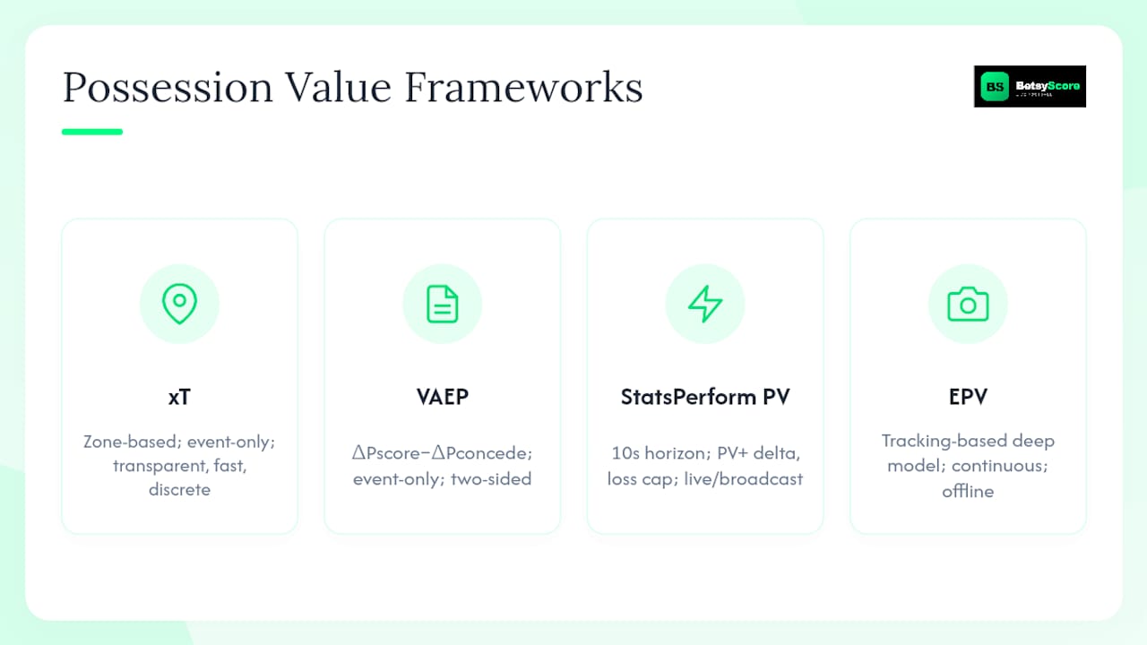
Four implementations define the practical landscape for analysts:
StatsPerform / Opta PV (time-based): The target variable is the probability of scoring within the next 10 seconds of possession. This time-based horizon improves interpretability and empirical performance for live applications. PV+ is the before/after delta, and a loss cap limits excessive negative credit. Output formats include per-action PV+, player PV+ leaderboards, and match-level possession quality scores. Best suited for live pipelines and broadcast-facing products.
VAEP (action-based, two-sided): Values each action as ΔPscore − ΔPconcede over the next k actions. The two-sided design gives defenders credit for game-saving actions and penalizes risky plays that raise conceding odds. VAEP runs on event data only, making it accessible across competitions. It is the most widely replicated open framework in academic soccer analytics.
EPV (Fernandez, Bornn, Cervone — deep learning): The SSAC paper presents a fine-grained EPV framework using learned sequence and state representations from tracking data. The model estimates possession outcomes continuously, not just at action moments, enabling smooth EPV timelines across a possession. Computationally intensive; best suited for offline analysis and research.
xT (location surface, Singh): Divides the pitch into zones and credits ball-movement between zones. Transparent, fast, and reproducible with event data. Blind to pressure, action type, and sequence context. Useful as a teaching tool and for quick pitch-value surfaces, but not a substitute for full PV in production scouting.
The practical differences come down to three axes: interpretability (xT > VAEP > StatsPerform PV > EPV), data requirements (xT and VAEP need event only; EPV needs tracking), and output granularity (EPV is continuous; others are discrete per-action).
How do you evaluate and validate a possession value model?
Primary evaluation metrics
- Brier score: Mean squared error between predicted probability and binary outcome. Lower is better; a Brier score near the naive baseline (always predicting the base rate) signals a model that has learned nothing useful.
- Log loss: Penalizes confident wrong predictions more heavily than Brier. Use both together; a model can look acceptable on Brier while being poorly calibrated on log loss.
- Calibration curves: Plot predicted probability bins against observed scoring rates. A well-calibrated model’s curve lies close to the diagonal. Calibration drift across competitions (e.g., a model trained on Premier League data applied to MLS) is a common failure mode.
- Rank-based metrics: Spearman correlation between model-ranked actions and human-expert rankings for a held-out action set. Useful for scouting applications where relative ordering matters more than absolute probability.
Validation checklist
- Split data by season or match block, not randomly by action. Random splits leak future information into training.
- Train on seasons N−2 and N−1; validate on season N. Repeat with a rolling window.
- Run calibration tests stratified by competition, match phase (open play vs. set piece), and score state. A model calibrated overall can be badly miscalibrated in specific subgroups.
- Perform ablation studies: remove one feature group at a time and measure the drop in Brier score to identify which inputs drive performance.
- Stress-test with downsampled tracking data (simulate event-only conditions) to understand how much performance degrades without full tracking.
- Check for calibration drift by applying the model to a held-out competition and plotting calibration curves separately.
Industry practice recommends combining model outputs with video review for any high-impact decision, such as a transfer recommendation or tactical system change. No PV model is a substitute for contextual judgment.
What are the practical applications of PV in scouting and tactics?
PV outputs translate into concrete workflows across several domains:
- Player recruitment: Rank players by PV+ per 90 across leagues to surface undervalued creators and defensive contributors. A midfielder with high PV+ in a lower-division league is a candidate for further video review, not an automatic signing.
- Tactical analysis: Aggregate PV+ by action type and pitch zone to identify which patterns (e.g., switches of play, third-man runs) generate the most value for a given team. This is more precise than pass-completion rates or touch maps alone.
- In-match decision support: Live PV surfaces updated every few seconds show which team is controlling possession quality, not just possession percentage. Substitution timing and pressing triggers can be informed by real-time PV trends.
- Broadcast visualization: EPV timelines showing how possession value rises and falls across a sequence make model behavior interpretable to coaches and broadcast audiences. Research figures from the Fernandez et al. work demonstrate how these visualizations expose the moments of highest leverage in a possession.
- Match prediction pipelines: PV aggregates (average PV per possession, PV differential) feed into probabilistic match-outcome models as features alongside xG, form, and head-to-head records. Understanding how football stats are calculated at the event level is a prerequisite for building these pipelines correctly.
For live applications, PV feeds into match prediction algorithms that update win probabilities in real time as possession quality shifts. The combination of PV and xG gives prediction models a richer signal than either metric alone.
What are the known limitations of possession value models?
Data quality risks
- Missed or mislabeled events in the source data propagate directly into PV+ values. A missed tackle or an incorrectly attributed pass changes which player receives credit.
- Tracking dropout (lost player IDs, frame gaps) degrades pressure features and can produce spikes in PV estimates that do not reflect real game states.
- Event data coverage varies by competition. Models trained on top-five European leagues may not calibrate well when applied to lower divisions or international tournaments with different data providers.
Statistical pitfalls
- Volume bias: Touch-heavy players accumulate PV+ mechanically. A central midfielder who receives 80 passes per match will show higher gross PV+ than a winger who receives 30, even if the winger’s per-action value is higher. Always normalize.
- Calibration drift: A model trained on one season or competition can drift out of calibration when applied to another. Tactical shifts, rule changes, and data-provider updates all affect the underlying distribution.
- Correlation vs. causation: High PV+ in a zone does not mean the team’s tactic of playing through that zone causes wins. Teams that are already winning tend to play in higher-value zones because the game state allows it.
Mitigation strategies
Pro Tip: *Apply possession-adjusted rates rather than raw per-90 figures when comparing players across teams with very different possession styles.
Additional guardrails include minimum-appearance filters before ranking, periodic recalibration of the scoring model against new seasons, and always pairing PV outputs with video review for high-stakes decisions.
How do you build a PV model from scratch?
Implementation checklist
- Acquire event data. Obtain structured event logs (Opta, StatsBomb, or equivalent) with action type, timestamp, x/y coordinates, team, player, and outcome. Confirm possession segmentation rules with the data provider.
- Segment possessions. Define possession boundaries: a new possession starts on a change of ball control, a ball out of play, or a goalkeeper restart. Label each action with its possession ID.
- Construct labels. For each action, scan forward within the horizon window (e.g., 10 seconds or next 10 actions). Set Pscore = 1 if the team scores within that window; Pconcede = 1 if the opponent scores.
- Engineer features. Compute x/y location, distance and angle to goal, action type (one-hot), time in match, score differential, and possession sequence position. Add pressure features if tracking data is available.
- Handle class imbalance. Goals are rare. Use class weights in the loss function or apply SMOTE-style oversampling on the minority class.
- Select and train the model. Start with gradient-boosted trees (XGBoost or LightGBM). Tune via cross-validation on a season-level holdout.
- Calibrate probabilities. Apply isotonic regression or Platt scaling to the model’s raw outputs. Check calibration curves stratified by competition and match phase.
- Evaluate. Compute Brier score, log loss, and calibration curves on a held-out season. Run ablation studies.
- Deploy for live inference. For near-live PV, pre-compute state features from the event stream and serve predictions via a lightweight REST API. Target latency under 500 milliseconds per action for broadcast-facing applications.
- Monitor and recalibrate. Track calibration drift monthly. Retrain or recalibrate when the model’s predicted probabilities diverge from observed rates by more than a defined threshold.
Starter pipeline sketch
| Stage | Input | Output | Tool |
|---|---|---|---|
| Possession segmentation | Raw event log | Possession-labeled events | Python / pandas |
| Feature engineering | Labeled events | Feature matrix | scikit-learn, NumPy |
| Label construction | Feature matrix + horizon | Pscore / Pconcede labels | Custom Python |
| Model training | Feature matrix + labels | Trained classifier | XGBoost / LightGBM |
| Calibration | Raw probabilities | Calibrated PV scores | scikit-learn CalibratedClassifierCV |
| Evaluation | Calibrated scores + labels | Brier, log loss, calibration curves | scikit-learn metrics |
| Serving | Live event stream | Per-action PV+ in near-real time | FastAPI / Flask |
Pro Tip: Once your event-only baseline is validated and calibrated, the highest-value upgrade is adding pressure features derived from tracking data. Pressure at the moment of action is the single feature most likely to improve calibration in tight game situations, based on the design choices documented in the Fernandez et al. EPV framework.
An analyst’s perspective on what actually matters in production
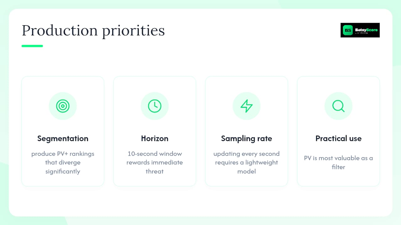
The academic literature on PV and EPV is rich, but production realities impose constraints that papers rarely address. The most consequential design choice is not the model architecture; it is the possession segmentation rule. Two teams using different segmentation conventions can produce PV+ rankings that diverge significantly for the same player, even when both models are well-calibrated. Analysts who skip this step and compare outputs across vendors are comparing different quantities.
The second underappreciated issue is the horizon. A 10-second window, as used in StatsPerform’s framework, rewards actions that create immediate threat. A longer horizon rewards patient build-up. Neither is wrong, but they answer different questions. Choosing the horizon should follow the use case, not convenience.
For live platforms, the tradeoff between sampling rate and compute cost is real. Updating PV every second requires a lightweight model; updating every 10 seconds allows more complex state representations. Betsyscore’s approach prioritizes low-latency PV surfaces for live users, feeding into AI-powered match predictions that update win probabilities as possession quality shifts in real time. The result is a momentum signal that reflects not just who has the ball but how dangerously they are using it.
The most common misuse of PV in practice is treating it as a standalone ranking tool without context. A player’s PV+ leaderboard position means very little without knowing the team’s possession style, the competition’s data quality, and the sample size. PV is most valuable as a filter, narrowing a scouting list from hundreds of players to a shortlist worth video review, not as a final verdict.
Sources
The sources below are the primary references for the concepts and implementation guidance in this article:
- A framework for the fine-grained evaluation of … (EPV paper)
- Introducing a Possession Value framework
- What Is Possession Value (PV)?
- Possession Value and VAEP Explained: Scoring Every Action on the Pitch — SoccerAnalytics
- What is Expected Threat (xT)? Possession Value models explained
FAQ
What is possession value in soccer analytics?
Possession value (PV) measures how much each on-ball action increases or decreases a team’s probability of scoring during that possession, expressed as a per-action delta called PV+. It assigns a quantified value to passes, carries, tackles, and dribbles, not just shots.
What does PV mean in football statistics?
PV stands for Possession Value, the probability that a team in possession will score within a defined horizon. PV+ is the change in that probability caused by a specific action, calculated as PV(state after action) minus PV(state before action).
What is EPV in soccer, and how does it differ from PV?
EPV (Expected Possession Value) is the deep-learning implementation of the PV concept developed by Fernandez, Bornn, and Cervone, which estimates possession outcomes continuously using learned sequence representations from tracking data. Standard PV frameworks compute a discrete value per action; EPV produces a smooth probability curve across the entire possession.
What is the 4-3-3 possession tactic, and how does PV measure it?
The 4-3-3 is a formation that prioritizes wide attacking play and high pressing, generating possession sequences through the flanks and into central areas. A PV model quantifies which specific actions in those sequences (e.g., switches of play, third-man combinations) add the most scoring probability, making it possible to compare the value of different 4-3-3 patterns across teams.
How is possession value different from expected goals (xG)?
xG assigns a scoring probability only to shots, making it a finishing-quality metric. PV assigns a value to every action in the possession, crediting the build-up play, defensive recoveries, and creative sequences that xG cannot see. The two metrics are complementary: xG measures shot quality; PV measures how the team got there.