Turn xG vs xGA into Live Signals After 8–10 Matches for Analysts
Expected goals (xG) measures the quality of chances a team creates; expected goals against (xGA) measures the quality of chances it allows. Use xG to judge whether a team’s attack is generating real scoring chances or living off luck. Use xGA to judge whether its defense is sustainable or riding a hot goalkeeper. Compare the two together, and you get a clearer read on whether results match performance.
TL;DR:
- Teams with high xG but low goals scored may improve their finishing efficiency over time, especially if the pattern persists across several matches.
- Defensive xGA offers insights into true defensive strength independent of goalkeeping form, but models differ by data provider, so comparisons require caution.
- Per 90 statistics for xG and xGA allow better comparisons between players and teams with varying amounts of playing time, reducing bias from injuries or rotations.
- Variance in xG and xGA results is common in single matches, so short-term anomalies should be viewed as noise unless confirmed over a multi-game sample.
- Live tracking tools like Betsyscore provide real-time updates of xG and xGA, helping viewers interpret the momentum and pressure during ongoing matches.
Table of Contents
- xG vs xGA: The Core Definitions
- How xG and xGA Are Actually Calculated
- Reading xG and xGA Together: What Analysts Actually Do
- Where xG and xGA Can Mislead You
- What the Numbers Look Like in a Real Season
- How Betsyscore Applies These Numbers in Real Time
- Where xG and xGA Came From
- Putting xG and xGA to Work on Teams and Players
- Why Tactics Change the Numbers
- Where xG and xGA Fit Among Other Analytics Metrics
- How Coaches Use These Numbers to Make Decisions
- When to Trust the Numbers and When to Watch the Tape
- Try BetsyScore for Live xG and xGA Application
- Sources
- FAQ
xG vs xGA: The Core Definitions
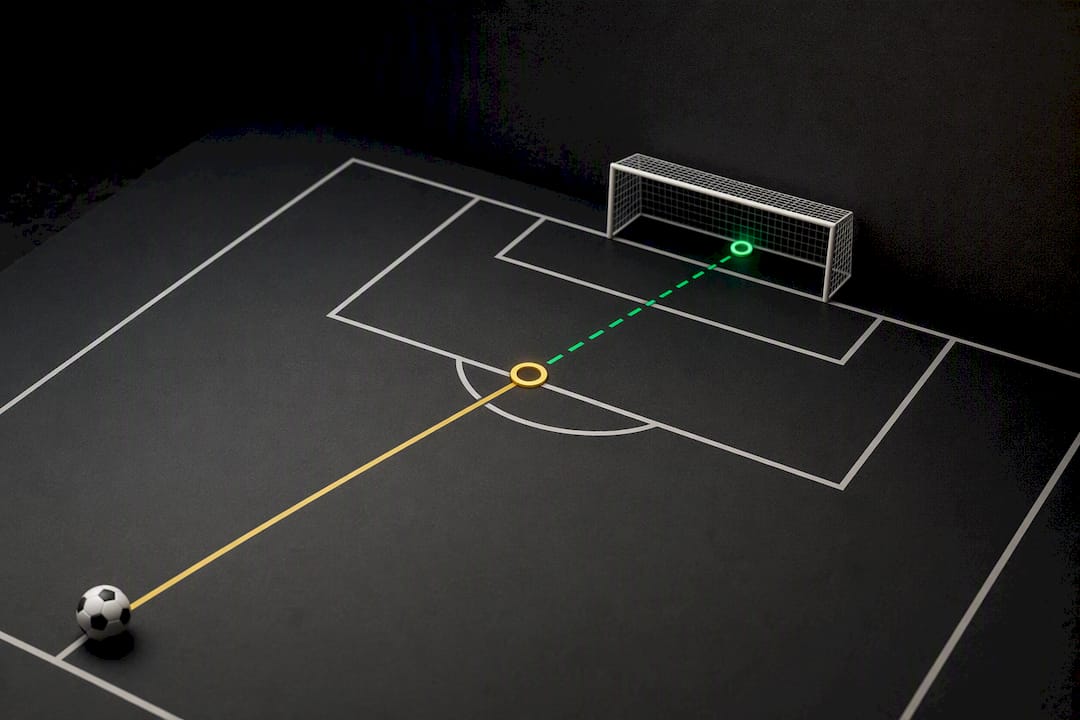
Expected goals assigns every shot a probability between 0 and 1, representing the estimated chance that specific shot becomes a goal, based on where it was taken, the angle, and the situation around it. Add up those probabilities across a match, and you get a team’s xG total. xGA works the same way, but it sums the probabilities of shots a team faces, not takes.
Here’s a simple way to see the split. Imagine a striker takes a shot from six yards out with no defender nearby. A speculative strike from 30 yards might carry an xG of 0.02. If a team takes both shots, its match xG is 0.47. If its opponent generates two similar shots against it, that same 0.47 becomes the opponent’s xGA.
Analysts also track xG per 90 and xGA per 90 to compare players and teams across different amounts of playing time, since raw totals get distorted by injuries, rotation, or games missed.
The distinction matters most in what each metric measures:
- xG reflects the quality of chances your team creates.
- xGA reflects the quality of chances your team allows.
- Neither one cares whether the ball actually went in.
xGA is specifically built to expose defensive quality independent of goalkeeping form, and it’s used across analytics circles as a proxy for how much danger a defense concedes, not just how many goals it lets in.
How xG and xGA Are Actually Calculated
Every xG model runs on a set of shot level inputs, and the exact recipe varies by data provider. The common variables include:
- Shot location and distance from goal
- Shot angle relative to the goal frame
- Body part used (foot, head, other)
- Assist type (through ball, cross, cutback, rebound)
- Defensive pressure at the moment of the shot
- Goalkeeper positioning
Providers don’t all weigh these the same way. Some incorporate defender positioning or passing sequences before the shot; others stick to a leaner model. Because xG models differ by provider, the same shot can score differently depending on whose numbers you’re reading, which means you should never treat an xG figure from one site as directly comparable to one from another without checking methodology.
One useful companion metric here is PSxG, or post-shot expected goals. Instead of grading a shot the instant it’s taken, PSxG recalculates the danger of a shot after it’s struck, factoring in placement and power once the ball is actually on target. That distinction lets analysts isolate a goalkeeper’s shot-stopping performance from the defense in front of them. If a keeper consistently allows fewer goals than PSxG suggests they should, that’s a real shot-stopping signal, not just good luck.
Reading xG and xGA Together: What Analysts Actually Do
Put xG and xGA side by side and you get xG differential (xGD), calculated as xG minus xGA. A positive xGD over a sustained stretch usually points to a team that’s outplaying opponents on both ends of the field, regardless of what the league table says at a given moment.
Analysts lean on the pairing in a few practical ways:
- Spot finishing variance. A team generating strong xG but scoring fewer actual goals is either finishing poorly or getting unlucky. Which one it is usually only becomes clear over several matches.
- Flag defensive fragility. A team with persistently high xGA but few goals conceded is likely riding strong individual goalkeeping. That tends to regress toward the defense’s true quality as the sample grows.
- Scout for style, not just output. Comparing a player’s or team’s shot locations against their xG profile reveals whether they’re generating dangerous positions or forcing low-probability attempts.
- Preview matches with context. Pairing a team’s attacking xG with an opponent’s defensive xGA gives a more grounded expectation than looking at recent scorelines alone.
Where xG and xGA Can Mislead You
xG and xGA are probabilistic tools, not verdicts. A shot rated at 0.30 doesn’t score three times out of ten in any predictable pattern. It’s an estimate drawn from thousands of similar shots, and any single match can land far from that average through pure variance.
The models also miss things that matter. They don’t fully account for exceptional individual finishing, a moment of pure improvisation, or a wonder strike that no location-and-angle formula would ever flag as likely. Similarly, xG treats a diagnostic signal as if it were predictive far too often. One match’s xG tells you what happened; it doesn’t reliably tell you what happens next unless the pattern repeats across several games.
Before trusting any xG or xGA figure, run through a short checklist:
- Confirm which provider generated the number and whether it discloses its model inputs.
- Check the sample size. A handful of matches is noise; a full season is signal.
- Compare xGA against PSxG to separate defensive quality from goalkeeping form.
- Avoid mixing numbers from two different providers in the same comparison.
Pro Tip: When you see a shocking xG total after just two or three matches, ignore it. Wait for a team to cross the 8 to 10 game mark before treating the number as anything more than early noise.
What the Numbers Look Like in a Real Season
Manchester City’s 2023/24 season provides a clean illustration of how xG and actual results diverge even for elite teams. City posted an xG of 89.55 against 86 actual goals scored, a gap of roughly 3.5 goals below model expectation. On the defensive side, their xGA sat at 37.27 against 34 goals actually conceded, meaning they allowed about 3 fewer goals than the model predicted they would.
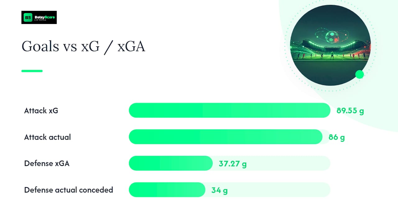
Neither gap is dramatic, but both show the same lesson: even a squad stacked with elite finishers and a well drilled defense won’t match its xG numbers exactly. The attack underperformed its shot quality slightly; the defense overperformed its expected concessions slightly, likely a mix of goalkeeping and finishing variance on the opponents’ side.
At the match level, this shows up constantly. A team can out-xG its opponent 2.1 to 0.6 and still lose 1 to 0 off a single defensive mistake or a moment of brilliance. When that happens, look past the scoreline and ask:
- Did the losing team generate the higher quality chances?
- Was the winning goal a low probability shot that simply landed?
- Is this a one-off or part of a repeating pattern across recent matches?
If the pattern repeats over multiple games, it’s worth acting on. If it’s isolated, treat it as one unlucky night.
How Betsyscore Applies These Numbers in Real Time
Every xG model is built differently, which is exactly why raw numbers from separate sources rarely line up cleanly. Some platforms combine expected goals data with recent form and head-to-head history, producing win-probability percentages that account for more than a single shot quality snapshot.
That approach shows up across some platforms in a few concrete ways: live scores that update frequently, a minute-by-minute momentum read that shows which side is generating pressure right now, detailed player profiles, and tournament leaderboards spanning many competitions. For readers who want to go deeper into the mechanics behind these numbers, the guide on how football stats are calculated walks through the modeling choices behind the data.
Where xG and xGA Came From
Expected goals didn’t start as a mainstream football metric. Its roots trace back to shot-quality models used in ice hockey analytics during the 2000s, where analysts were already trying to separate scoring chances from finishing luck. Football analysts adapted the underlying idea, building shot-location datasets and probability models specific to the sport’s geometry and playing patterns.
Public adoption accelerated through the 2010s as data companies began publishing shot maps and match-level xG figures on accessible platforms. Sites like FBref started making xG and xGA numbers freely browsable, which pulled the metric out of private analytics departments and into mainstream match commentary and post-game debate.
xGA followed a slightly different path. Early expected goals work focused almost entirely on attack, since the original question was “how many goals should this team have scored?” Applying the same shot-probability logic to the defensive side of the ball, tallying the quality of chances conceded rather than created, came later, as analysts realized the same math could isolate defensive performance from a hot or cold goalkeeper.
By the mid 2010s, broadcasters began displaying live xG figures during televised matches, and by the 2020s, xG and xGA had become standard columns in league tables, scouting reports, and fantasy football tools. What started as a niche hockey borrowed concept is now baked into how most fans read a match report.
Putting xG and xGA to Work on Teams and Players
Team level analysis leans on xG and xGA to answer a question that goals alone can’t: is this team’s underlying performance actually improving, or is the scoreline just flattering them? A club climbing the table while its xGD trends downward is a warning sign worth watching, even if the standings look fine for now.
Player level applications get more granular. Strikers get evaluated on non-penalty xG per 90, which strips out penalty conversions to isolate open-play shot quality. A forward outscoring their xG consistently across multiple seasons is showing genuine finishing skill rather than a hot streak, since the sample size rules out most of the variance explanation.
Midfielders and wide players get judged on xG assisted (xGA in the passing sense, sometimes labeled xA), which measures the quality of chances created for teammates rather than shots taken personally. This distinguishes a player who racks up assists from good fortune versus one who consistently sets up high quality chances regardless of whether the finish lands.
On the defensive side, individual center backs and defensive midfielders get evaluated on how their presence shifts team xGA when they’re on the field versus off it. A defender whose team’s xGA spikes in their absence is contributing something the raw tackle and interception counts don’t capture. Betsyscore’s player profile pages surface this kind of underlying data alongside traditional box score numbers, giving a fuller picture than goals and assists alone.
Why Tactics Change the Numbers
Playing style shapes xG and xGA independent of raw quality. A team built around high pressing and quick transitions tends to generate shots from central, high probability areas because turnovers happen closer to the opponent’s goal. That style pushes attacking xG up almost mechanically, separate from how skilled the finishers actually are.
Compare that to a team built around patient possession and wide overloads. That approach often produces a higher shot volume but from wider angles, which can inflate the number of attempts while keeping average shot quality lower. Two teams can post similar total shot counts and wildly different xG totals because of where those shots come from.
Defensive tactics work the same way in reverse. A low block that concedes possession but compresses space centrally often keeps opponent shots to the perimeter, holding xGA down even against dominant opponents. A high defensive line that presses aggressively higher up the field can suppress shot volume entirely, but when it gets broken, it tends to concede clearer, higher probability chances, which shows up as spikes in xGA even if the overall goals conceded total looks fine.
This is why comparing xG or xGA across teams with fundamentally different systems needs context. A counter-attacking side with modest xG numbers isn’t necessarily a weaker attacking team than a possession heavy side with inflated shot volume. It’s a different approach to creating the same outcome, and the raw numbers alone won’t tell you which is working better without watching how the chances are actually generated.
Where xG and xGA Fit Among Other Analytics Metrics
xG and xGA sit inside a wider family of advanced football metrics, and understanding how they relate helps you avoid over relying on any single number. Expected points (xP) takes team level xG and xGA and projects them forward into likely match outcomes and points totals, giving a longer range view of whether a team’s league position matches its underlying performance. Betsyscore’s explainer on expected points breaks down how that projection actually works.
Expected threat (xT) measures the value of ball progression on the field, rewarding passes and dribbles that move play into dangerous zones, even when they don’t directly lead to a shot. Where xG only grades the shot itself, xT credits the buildup that got a team into position to take it.
PPDA (passes per defensive action) measures pressing intensity by counting how many passes an opponent completes before a defensive team makes a tackle, interception, or foul. It’s a useful companion to xGA because it explains part of why a team’s defensive shot quality looks the way it does.
None of these metrics replace xG or xGA. They contextualize them. A team with strong xT but weak xG might be excellent at reaching dangerous areas but poor at converting positions into actual shots, a distinction that pure xG numbers can’t reveal on their own.
How Coaches Use These Numbers to Make Decisions
Professional coaching staffs use xG and xGA as diagnostic tools during and after matches, not just as postmortem talking points for broadcasters. In game, some clubs track live xG trends to judge whether a tactical setup is generating the shot quality they expected, and substitutions sometimes follow directly from that read, pulling a winger who isn’t threatening the box in favor of one who might.
Post-match, staff review shot maps alongside xG to separate execution problems from selection problems. If a team is generating high quality chances but missing them, the fix might be finishing drills rather than a formation change. If the underlying chance quality is poor despite plenty of possession, the issue is more likely tactical: wrong areas of the field, poor movement in the box, or a buildup pattern that isn’t breaking defensive lines.
On the defensive side, a rising xGA trend over several matches often triggers a tactical review before it shows up as goals conceded, since the shot quality data usually moves before the results do. Staff might tighten a defensive line, adjust pressing triggers, or rotate personnel based on which players are on the field when opponent xGA spikes.
Recruitment departments lean on the same logic longer term, using multi season xG and xGA data to identify players whose underlying numbers suggest untapped value, or to flag players whose output has been propped up by unsustainable finishing variance.
When to Trust the Numbers and When to Watch the Tape
xG and xGA work best as diagnostic tools, not crystal balls. The most reliable use case treats them as one input among several, cross checked against PSxG for goalkeeper evaluation and against actual shot maps or match video when a number looks surprising.
A single game’s xG differential rarely tells you anything definitive. A run of eight or ten matches usually does. Build the habit of checking xG and xGA alongside shot counts rather than trusting one headline figure, and use the vetting checklist above every time a new provider’s numbers show up in your feed.
— Aria
Try BetsyScore for Live xG and xGA Application
Reading xG and xGA in a table after the final whistle is one thing. Watching how those numbers shift while a match is still live is another experience entirely, and it’s where Betsyscore fits into your routine.

Betsyscore turns the same expected goals concepts covered above into live, usable signals. Its AI-powered match predictions blend expected goals with recent form and head-to-head history into a single win-probability read, updated as the match develops rather than frozen at kickoff. Pair that with the minute-by-minute momentum tracker, and you can watch in real time whether a team’s shot quality is actually building pressure or just accumulating empty possession. Coverage runs across many top leagues and more than 200 competitions worldwide, so the same interpretation habits from this article apply whether you’re watching a title race or an international qualifier.
Head to Betsyscore’s live scores page during your next match and check the momentum read against the shot quality you’re seeing on screen. It’s the fastest way to turn the theory above into something you actually use.
Sources
- Decoding Expected Goals (xG) & Expected Goals Against (xGA)
- Expected Goals Against (xGA) – Football Statistics Explained - The Football Analyst
- Expected goals
- xG explained (FBref)
FAQ
What Does xGA Stand For?
xGA stands for expected goals against, which totals the probability of every shot a team faces becoming a goal, used to judge the quality of chances a defense allows rather than just goals conceded.
Why Is xG Considered Flawed by Some Analysts?
xG is a probabilistic estimate, not a guarantee, so it can’t fully account for exceptional finishing, unpredictable moments, or provider-specific modeling differences that make numbers hard to compare across data sources.
What xG Counts as a Big Chance?
There’s no single universal threshold, but shots with a relatively high xG value are generally treated as high quality chances, representing a significant probability of scoring based on location, angle, and situation.
Is a Higher xG Always Better?
A higher xG generally signals better chance creation, but it only becomes meaningful when read alongside actual goals scored and sustained across multiple matches rather than judged from a single game.
Where Can I Check Live xG and xGA During a Match?
Public stats sites publish post-match xG data, but for a live, in-match read paired with win probability, Betsyscore’s live scores and prediction pages update figures as the match unfolds.